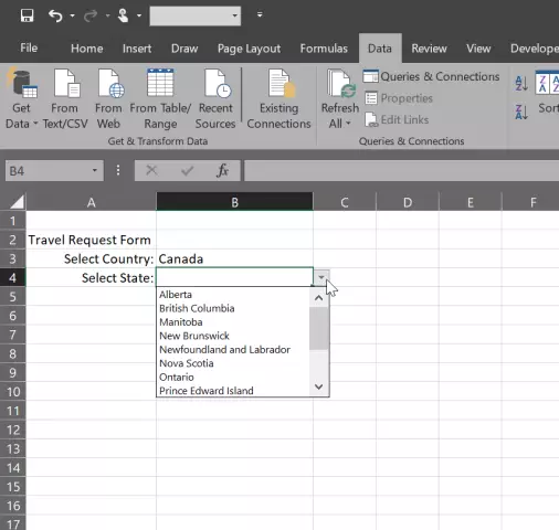
Filling an Excel document using drop-down lists can significantly speed up and simplify work with tables. Dropdown lists are useful when working with persistent or infrequently changing data. It is enough to create a data set once, so that the further filling of the document is carried out almost automatically.
Method 1. Quick dropdown list
The fastest way to create a drop-down list in Excel is by using the Select from Drop-Down List function in the cell's context menu. Its principle of operation resembles the usual Excel autocomplete.
First, you need to enter a list of categories of the future list in the column one by one, without skipping empty cells. In the next cell, you need to set the cursor and call the context menu by clicking on the "Select from the drop-down list" field. It is even easier to call the drop-down menu by pressing the "Alt" + "Down Arrow" keys.
This method is suitable only for data entered strictly within one column and without skipping cells.
Method 2. Universal
A more versatile way to create a drop-down list in Excel will require more manipulation, but at the same time it allows you to solve more complex problems.
First, you need to select a range with a list of categories of the future list. The further sequence of actions depends on the version of the program.
In Excel 2007 and higher, in the "Formulas" field, click on "Name Manager" - "Create". In the dialog box that opens, you must enter a name, taking into account the fact that it must begin with a letter and not have spaces. After completing the entry, you must click on "OK".
You can do it even easier - after selecting a range, changing the name is available in the corresponding field located to the left of the function line, where the cell address is usually indicated. After entering the name of the range, be sure to press "Enter".
In earlier versions of Excel up to 2003, you must select "Insert", then click "Name" and select "Assign". Further sequence is unchanged.
Now you need to select the range of cells to which the created list will belong. For this, an area of cells is selected, the "Data" tab opens, in which you need to select the "Data Validation" function. In the opened dialog box, in the "Parameters" tab, in the "Data type" field, set "List". In the "Source" field that appears, click on "=" and enter the name of the created list. When you click on "OK", cells in the selected range, when you click on them, acquire a drop-down menu.
This method of creating a drop-down list in Excel is good for categories that are fixed in terms of the number of categories with the realized ability to change their name.


