Microsoft Excel is a spreadsheet tool and therefore presents data in a tabular format by default. The creation of a table in this application is carried out in just two steps: data entry and border design. However, as in other MS Office applications, the desired result in Excel can be achieved in several ways.

Instructions
Step 1
Open Microsoft Excel by clicking on Start -> All Programs -> Microsoft Office. A new book will open: by default, it will be the "Book1.xlsx" file with three blank sheets laid out with a table grid.

Step 2
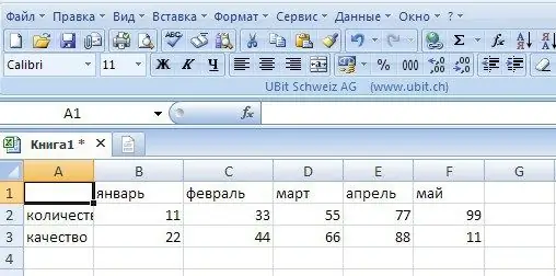
If you need to create a simple table for visual presentation of data on a third-party resource, for example, print, export it to Word or another application, you can immediately start entering data into columns in a regular format. Sign the column and row names, if necessary, and enter the data in the appropriate cells.
Step 3
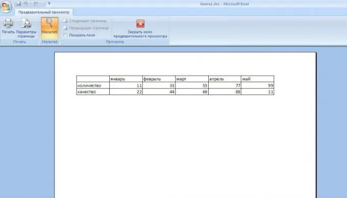
Now we need to adjust the width of the columns. You can do this manually by hovering the cursor over the right border of the desired column and stretching it with the mouse to the required width. You can set the columns to fixed widths, or you can choose the AutoFit by Content feature. To do this, select the columns to be formatted, and on the "Menu" tab, select "Format" -> "Column", and in the drop-down menu, select the desired option. You can see how your table will look when printed by selecting the preview button on the toolbar or by pressing Ctrl + F2.

Step 4
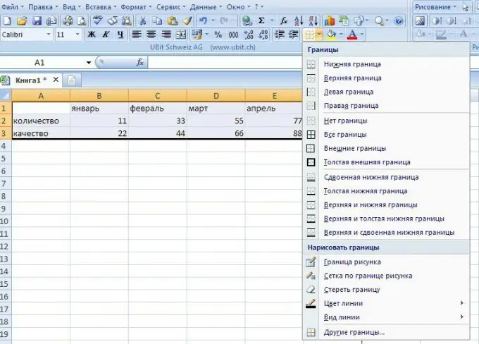
Now you need to draw the grid of the table so that it can be displayed on the print. To do this, select the table with the cursor and find the "Borders" button located to the right of the "Increase Indent" button on the toolbar. It will have a different name and look, depending on which tool was used earlier. However, this is usually a dotted square with an arrow on the right, clicking on which opens a menu of available tools.
Step 5
Select the "All Borders" item from the menu to draw all the cells on each side, or use any necessary tool from the list at your discretion. Please note that the "Draw Borders" tool group contains not only buttons for drawing or erasing lines (pencil and eraser, respectively), but also options for choosing the type and color of lines.
Step 6
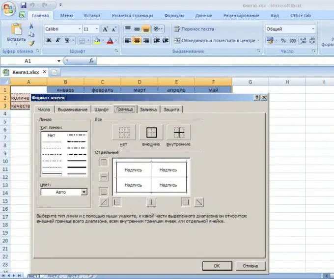
Another way to draw a table on top of already entered data is to use the Format Cells tab in the right-click drop-down menu. To do this, use the cursor to select a cell or a group of cells with data, the format of which you want to change, right-click and select "Format cells". In the window that opens, select the "Border" tab. On this panel, you can simultaneously select the appropriate type and color of lines, indicate to which part of the selected range to apply the lines, and immediately see the result in the viewport.
Step 7
Here, on the "Alignment" tab, you can set parameters for the placement of content in cells, such as "display", "direction" and "orientation" of the text. And on the "Font" and "Fill" tabs, you can select the required properties of the specified table parameters.
Step 8
When using the third method of drawing a table, data is entered into the already drawn grid last. In this case, first select the required range of cells on a blank sheet of paper.
Step 9
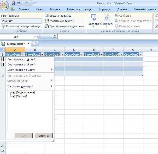
After that, on the toolbar, click on the "Insert" menu item, select the "Tables" mode. This operation can be done much faster by using the key combination CTRL + L or CTRL + T. In the window that appears, check the box "Table with headers". After that specify the names of the columns, otherwise they will be named "Column 1", "Column 2" and so on by default. To set the column names, place the cursor in the header cell and enter the name in the function bar.

Step 10
Use the controls to make changes to your spreadsheet in Excel. They can be found in the "Design" tab located on the toolbar. You can change the number of rows, columns, cell format, and more.

Step 11
Use the split sort feature to change only a portion of the table while keeping the rest as they were. To resize it, move the cursor over the dot mark in the lower right corner and drag to the side to offset the cell borders to give them new values.
Step 12
Contour the table. Then break the cells inside as you see fit. To increase the volume of one cell at the expense of another, use the button on the Merge Cells toolbar. You can also change the color of the font, cell background and other decorative elements that will help make your table look unusual and original. After you have set all the necessary parameters for the table design, start entering data. To make sure that your table looks exactly as you intended, you can use the "Print Preview" function, where, among other things, you can set page parameters for printing.


