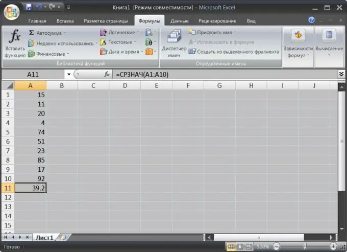
Microsoft Office Excel is the most common tool for working with tables for various purposes. To a large extent, its popularity is based on a fairly simple mechanism for working with formulas and the ability to use a large set of predefined mathematical, statistical, logical and other functions in them. Such formulas allow you to process tabular data in real time and generate complex resulting documents without knowledge of any programming language.

It is necessary
Microsoft Office Excel Spreadsheet Editor
Instructions
Step 1
Begin entering a formula into a cell in a spreadsheet editor by pressing an equal key. This sign at the beginning of a row tells Excel that it should interpret the contents of the cell as a formula, not tabular data.
Step 2
Use a / (slash) for division, * (asterisk) for multiplication, and ^ (circumflex) for exponentiation. For example, to multiply 2 by 3 and the result is cubed, click an empty cell in the table and type the following sequence of characters: = (2 * 3) ^ 3 When you finish typing, press Enter - Excel will calculate and show you the result. when entering formulas are indicated by their usual symbols.
Step 3
Insert cell references into formulas if tabular data needs to be used in calculations. To do this, when typing a formula, just click the desired cell in the table. For example, if cell A3 should show the result of multiplying the value in cell A1 by the value in cell A2, then click cell A3, enter an equal sign, click cell A1, enter a multiplication sign, click cell A2, and press Enter.
Step 4
Use the functions preset in the editor for more complex calculations in formulas. You can enter the function names yourself, but at first it is more convenient to use the "function wizard" dialog. For example, if you want to place the average value of a range of cells from A1 to A10 in cell A11, then click cell A10, press the equal sign, and then click the "Insert function" icon at the beginning of the formula bar above the table.
Step 5
Open the drop-down list "Category" in the appeared dialog box and select the line "Statistical". In the list of functions, click AVERAGE - it will be difficult to confuse, since the description of the selected function appears below the list.
Step 6
Click the "OK" button to go to the next step of the function wizard. In the second step, you need to specify the function parameters - each of them has its own set of parameters. To determine the average value of a range of cells, just set a link to its first and last cells in the "Number1" field. The wizard will insert the most probable range there, and you can change it if necessary.
Step 7
Click OK to complete the function wizard. This is a basic way to work with formulas and functions, and as you master it, you will discover a huge variety of use cases.


